Ahead of discussing how to calculate p value in excel, lets define it. In statistics, the p-value is the probability of obtaining results at least as extreme as the observed results of a statistical hypothesis test, assuming that the null hypothesis is correct.
A P-value less than 0.05 indicates strong evidence against the null hypothesis while a P-value greater than 0.05 indicates weak evidence against the null hypothesis.
Formula to Calculate P Value in Excel.
- In excel, click on data and choose data analysis.
- Select t-test:Paired Two Sample for Means.
- Add in the arguments, click OK and get your answer.
Example:
Calculate the P value of the gym program
| Name | Before (Weight in Kg) | After (Weight in Kg) |
| Mike | 54 | 53 |
| Alex | 60 | 64 |
| Esther | 92 | 70 |
| Ann | 52 | 47 |
| Cristiano | 70 | 64 |
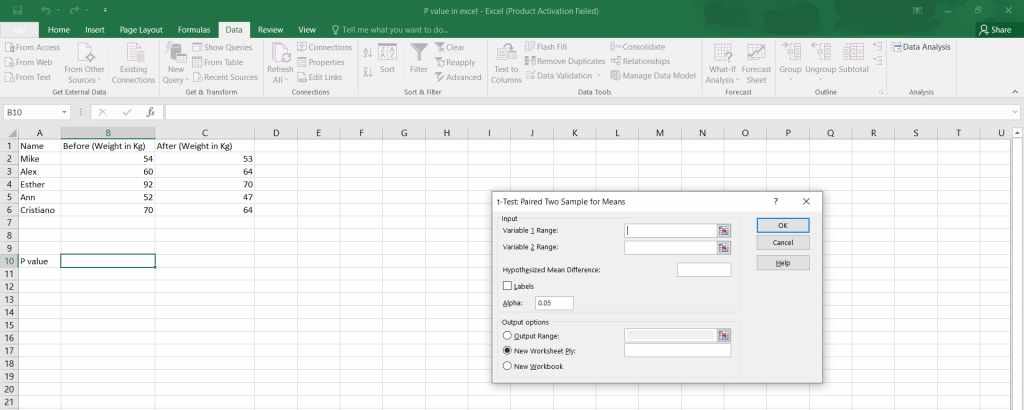
We begin by transferring the data to an excel spreadsheet.

Click on Data and choose data analysis,choose t-test:paired Two Sample for Means, input your arguments in the table that appears.

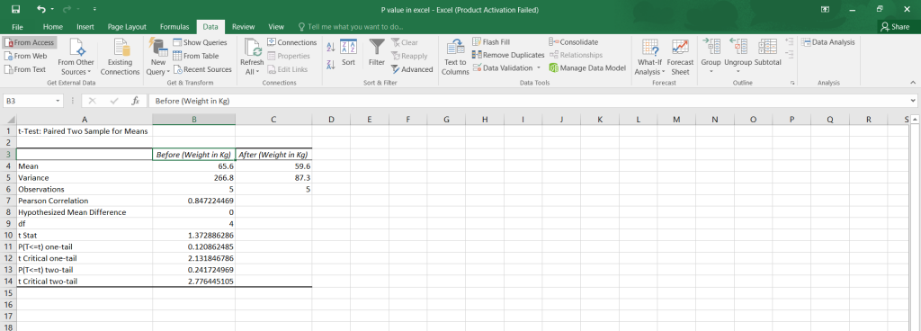
A new sheet like the one below will be formed with your results.

Therefore, on the results, we can see that the p-value with the one-tail test is 0.12 and the p-value with the two-tail test is 0.24.

